Tutorial: Creating 2D Meshes and Fitting to Data
In this tutorial we build a 2D mesh using cubic-Hermite elements and fit the mesh to data generated using a cosine function.
For this tutorial we’ll need to import scipy and morphic.
import scipy
import morphic
Building a Mesh
First, we create some node point which will be arranged in a regular 3x3
grid ranging from x = [-pi, pi] and y = [-pi, pi]. The z values
are set to zero.
# Generate a regular grid of X, Y and Z values
pi = scipy.pi
Xn = scipy.array([
        [-pi, -pi, 0],
        [  0, -pi, 0],
        [ pi, -pi, 0],
        [-pi,   0, 0],
        [  0,   0, 0],
        [ pi,   0, 0],
        [-pi,  pi, 0],
        [  0,  pi, 0],
        [ pi,  pi, 0]])
Because we are using cubic-Hermite element, the nodal values require derivative values which we default to,
deriv = scipy.array([[1, 0, 0], [0, 1, 0], [0, 0, 1]])
Now, we create the mesh,
mesh = morphic.Mesh()
We add the nodes where for each node value we append the derivative values,
for i, xn in enumerate(Xn):
    xn_ch = scipy.append(scipy.array([xn]).T, deriv, axis=1)
    mesh.add_stdnode(i+1, xn_ch)
Now we add four bicubic-Hermite elements, which are ['H3', 'H3']
basis,
mesh.add_element(1, ['H3', 'H3'], [1, 2, 4, 5])
mesh.add_element(2, ['H3', 'H3'], [2, 3, 5, 6])
mesh.add_element(3, ['H3', 'H3'], [4, 5, 7, 8])
mesh.add_element(4, ['H3', 'H3'], [5, 6, 8, 9])
And finally generate the mesh structures,
mesh.generate()
Generate Data
The data cloud is based on a cosine function, z = cos(x + 1) cos(y + 1).
A 200 x 200 grid of points are created in the x and y dimensions on which
the z values are generated. The res=24 parameter sets the
discretization of the elements. The higher the value the smoother the
rendered surface.
xd = scipy.linspace(-scipy.pi, scipy.pi, 200)
X, Y = scipy.meshgrid(xd, xd.T)
Xd = scipy.array([
        X.reshape((X.size)),
        Y.reshape((Y.size)),
        scipy.zeros((X.size, 1))]).T
Xd[:, 2] = (scipy.cos(Xd[:, 0])+1) * (scipy.cos(Xd[:, 1])+1)
Plotting
Here we want to view our initial mesh and data. First we need to extract the coordinates of the nodes (without derivatives) and a surface of the mesh, which is done using the following commands,
Xn = mesh.get_nodes()
Xs,Ts = mesh.get_surfaces(res=24)
Next we want to plot the mesh nodes and surface and the data which is
done using the morphic.viewer module,
from morphic import viewer
S = viewer.Scenes('MyPlot', bgcolor=(1,1,1))
S.plot_points('nodes', Xn, color=(0,1,0), size=0.1)
S.plot_surfaces('surface', Xs, Ts, color=(0.2,0.5,1))
S.plot_points('data', Xd[::7,:], color=(1,0,0), mode='point')
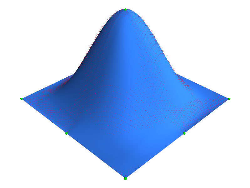
The resultant plot is shown where the nodes are plotted in green, the mesh surface in blue and the data in red,

Fitting
In this section we describe how to fit the mesh to the datacloud. Here
we use the fitting method that generates and solves a linear system of
equations, i.e., A.x = b, where A is the matrix of weights for
points on the mesh, x are the mesh parameters, and b are the
data point that the mesh points are fitted to. See TODO: add link
There are two demonstrations of the fitting process, first we fit without constraining mesh node parameters and second we fit with constraints on the node values and derivatives.
Fit Part 1: No Constraints
Ok, let’s get started. First we create a new fitting instance:
fit = morphic.Fit()
Then we add element points on the mesh to the fitting process. This is a 10x10 grid of points on each element. These are the points that will be projected to the datacloud.
Xi_fit = mesh.elements[1].grid(res=10)
for elem in mesh.elements:
    for xi in Xi_fit:
        fit.bind_element_point(elem.id, [xi], 'datacloud')
Then we generate the fit from the mesh. Here the fitting module will
calculate the weights for each grid point on the mesh and assemble these
in the A matrix for the A.x = b system.
fit.update_from_mesh(mesh)
We add the data cloud to the fitting process and call a function called
generate_fast_data which creates a kd-tree of the data for fast
searching of the closest data points.
fit.set_data('datacloud', Xd)
fit.generate_fast_data()
Now we invert the A matrix in order to speed up the fitting process and if the mesh to the datacloud. Currently we run the fit iteratively where each iteration involves finding the closest data points for the current mesh and then fitting the mesh to the closest data points. When the RMS error between the mesh and datacloud stops reducing or 1000 iterations are reached, then the fit will stop. These stopping criteria can be changed, see the details on the solve method.
fit.invert_matrix()
mesh, rms_err1 = fit.solve(mesh, output=True)
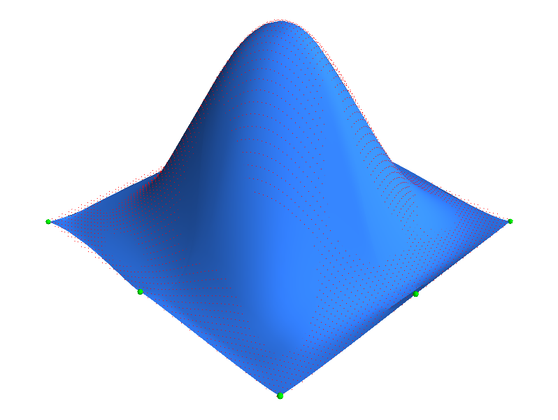
The plot of the resultant fit shows a fairly good fit except the boundaries are not straight and also we expect the middle node to be at the peak of the data cloud. This can be achieved in the fit by constraining the appropriate node parameters. This is described in the next section.
Fit Part 2: With Constraints
In this section we are going to constrain appropriate node values and derivatives to get straight boundaries and a more symmetric mesh. We define constrains on nodes values using the following command:
fit.bind_node_value(node_id, field_num, component_num, data_label, weight=weight)
where the weight defines the weighting of the constraint. The default
is 1, which is what the binding for the element points is set to. The
higher this number the closer the resultant fit will met its constraint.
Warning
Setting the weight very high compared to the minimum weight in the fit
can cause fitting issues.
Note
The indexing of the field_num and component_num starts at zero.
Just like how we added the data cloud, the data values we would like to constrain the node parameters to are defined using a data label. First we define an array of data labels indicating which how each node is constrained. The rows in the array represent the node and the columns represent x, y and z values. This allows a easy programatic way of setting the constraints. First, the node values are constrained, then the derivatives.
fix_nodes = [
        ['-pi', '-pi', 'zero'],
        ['zero', '-pi', 'zero'],
        ['pi', '-pi', 'zero'],
        ['-pi', 'zero', 'zero'],
        ['zero', 'zero', 'four'],
        ['pi', 'zero', 'zero'],
        ['-pi', 'pi', 'zero'],
        ['zero', 'pi', 'zero'],
        ['pi', 'pi', 'zero']]

weight1 = 100
for i, fix in enumerate(fix_nodes):
    node_id = i + 1
    # Fix node values
    fit.bind_node_value(node_id, 0, 0, fix[0], weight=weight1)
    fit.bind_node_value(node_id, 1, 0, fix[1], weight=weight1)
    fit.bind_node_value(node_id, 2, 0, fix[2], weight=weight1)

    # Fix node derivatives
    fit.bind_node_value(node_id, 0, 2, 'zero', weight=weight1) # dx/dxi2=0
    fit.bind_node_value(node_id, 1, 1, 'zero', weight=weight1) # dy/dxi1=0
    fit.bind_node_value(node_id, 2, 1, 'zero', weight=weight1) # dz/dxi1=0
    fit.bind_node_value(node_id, 2, 2, 'zero', weight=weight1) # dz/dxi2=0

# Flattens the corners. Stops z from dipping below zero, d2z/(dxi1.dxi2)=0
weight2 = 100
fit.bind_node_value(1, 2, 3, 'zero', weight=weight2)
fit.bind_node_value(3, 2, 3, 'zero', weight=weight2)
fit.bind_node_value(7, 2, 3, 'zero', weight=weight2)
fit.bind_node_value(9, 2, 3, 'zero', weight=weight2)

fit.update_from_mesh(mesh)
In the final line, we regenerate the fit from the mesh after we define the node value constraints.
Next, as above, we add the data values we constrain the node values to and regenerate the fast data. In this case, no kd-tree is created since there is only one value per data label.
fit.set_data('pi', scipy.pi)
fit.set_data('-pi', -scipy.pi)
fit.set_data('zero', 0)
fit.set_data('four', 4.)
fit.generate_fast_data()
And again we invert the matrix and solve the fit,
fit.invert_matrix()
mesh, rms_err2 = fit.solve(mesh, output=True)
As shown in the resultant plot, the fit produces straigher boundaries and a symmetric mesh, i.e., the nodes are laid out in a regular fashion.