Tutorial: PCA Meshes
In this tutorial we build a 1D cubic-Hermite PCA mesh. The population of meshes used to create the PCA mesh is generated by modifying some nodal parameters using a Gaussian ditribution. The output from PCA of this population of meshes are used to create the PCA mesh.
For this tutorial we’ll need to import scipy, random, pylab,
mdp and, ofcourse, morphic.
Creating a Population of 100 Meshes
First, we create simple 1D cubic-Hermite mesh with two nodes and one element.
mesh = morphic.Mesh()
mesh.add_stdnode(1, scipy.zeros((2, 2)))
mesh.add_stdnode(2, scipy.zeros((2, 2)))
mesh.add_element(1, ['H3'], [1, 2])
mesh.generate()
Then we create a function to randomise six the mesh parameters:
def randomise_mesh(mesh):
    import random
    import scipy

    xa = random.gauss(-2.5, 1)
    xb = random.gauss(2.5, 1)
    ya = random.gauss(-0.1, 0.5)
    yb = random.gauss(0.3, 0.5)
    dya = random.gauss(0, 0.1)
    dyb = random.gauss(0, 0.2)

    mesh.nodes[1].values = scipy.array([[xa, 5], [ya, dya + dyb]])
    mesh.nodes[2].values = scipy.array([[xb, 5], [yb, -dya]])

    return mesh
An example of running this function a 100 times and plotting the results is shown in the figure below.

Performing PCA
Although PCA can be performed an any data, it is not good practice to perform PCA data with mixed units, which in our case is a cubic-Hermite mesh that has position and derivative values. To overcome this issue we will convert the cubic-Hermite mesh to a cubic-langrange mesh, which will preserve all information.
To perform PCA, we convert all our meshes to cubic-lagrange by evaluating
the field values at Xi 0, 1/3, 2/3, and 1. These values are stored in
a large array for PCA.
Npop = 100 # number in the population
Xp = scipy.zeros((8, Npop))

for i in range(Npop):
    mesh = randomise_mesh(mesh)
    Xp[:,i] = mesh.elements[1].evaluate(
            [[0], [1/3.], [2/3.], [1]]).flatten()
Then we use MDP to perform PCA and print out the average mesh, mode values, and variance for each mode,
pca = mdp.nodes.PCANode(svd=True)
pca.execute(Xp.T)
#~ print pca.avg    # Average mesh
#~ print pca.v    # The modes
#~ print pca.d   # Variance shows there are 6 significant modes.
Now we can create a mesh that uses the PCA results.
Creating a PCA Mesh
Morphic has a node class to manage PCA values as nodes. It knows how to evaluate the vlaues of the node given a set of weights.
There are 4 steps to creating a PCA mesh:
- add the PCA weights as a standard node
- add the PCA variance as a standard node
- add the PCA nodes which references weights and variance nodes
- add the elements which references the PCA nodes
For example,
pcamesh = morphic.Mesh()

pcamesh.add_stdnode('weights', [1, 0, 0, 0]) # Step 1: weights node

pcamesh.add_stdnode('variance', [1, 0.5, 0.2, 0.1]) # Step 2: variance node

# Step 3: add the pca node for each node
pcamesh.add_pcanode(1, xm1, 'weights', 'variance')
pcamesh.add_pcanode(2, xm2, 'weights', 'variance')
pcamesh.add_pcanode(3, xm3, 'weights', 'variance')

# Step 4: add elements...
pcamesh.add_element(1, ['L2'], [1, 2, 3])

pcamesh.generate()
:warning:
The first value of the weights and variance nodes should be set to 1
since it it multiplied with the mean values from the PCA.
For our case, we will initialise some values and create a new mesh
called pcamesh which will store and evaluate the PCA values,
pcamesh = morphic.Mesh()

Nnodes = 4 # number of nodes
Ndims = 2 # number of dimensions
Ncomps = 1 # number of components
Nmodes = 6 # number of modes
Now we add the weights values
weights = scipy.zeros((7)) # Average mesh plus 6 modes
weights[0] = 1.0 # the weight on the average mesh
pcamesh.add_stdnode('weights', weights, group='pca_init')
And the variance values which are square rooted so that the weights can be defined in terms of standard deviations,
variance = scipy.zeros((7)) # Average mesh plus 7 modes
variance[0] = 1.0 # Set to 1 for the average mesh
variance[1:] = scipy.sqrt(pca.d[:6]) # variance for the 7 modes
pcamesh.add_stdnode('variance', variance, group='pca_init')
The mode values are added as PCA nodes which reference the weights and variance nodes,
xn = scipy.zeros((Ndims, Ncomps, Nmodes+1)) # node values array
for i in range(Nnodes):
    idx = i * Ndims
    # Add a PCA node using the node values, weights and variance
    xn[:, 0, 0] = pca.avg[0, idx:idx+Ndims] # add mean values
    xn[:, 0, 1:] = pca.v[idx:idx+Ndims,:Nmodes] # add 7 mode values
    pcamesh.add_pcanode(i+1, xn, 'weights', 'variance', group='pca')
Finally we add the element and generate the mesh,
pcamesh.add_element(1, ['L3'], [1, 2, 3, 4])

pcamesh.generate()
We can now modify the values of the weights and analyse or plot the mesh. Whenever the weights are change the mesh must be updated to recalculate the PCA node values. For example,
pcamesh.nodes['weights'].values[2] = 1.3
pcamesh.update_pca_nodes()
To show the outputs of the PCA mesh, we plot the top 4 modes of the mesh for weights of -2, -1, 0, 1, and 2.
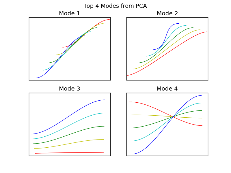
The python function used to plot these modes are below,
def plot_modes(pcamesh, mode, sp, title=None):
    colors = {-2:'r', -1:'y', 0:'g', 1:'c', 2:'b'}

    pcamesh.nodes['weights'].values[1:] = 0 # Reset weights to zero
    pcamesh.update_pca_nodes()

    pylab.subplot(sp)
    pylab.hold('on')
    # Plotting modes over a range of weights values
    for w in scipy.linspace(-2, 2, 5):
        pcamesh.nodes['weights'].values[mode] = w
        pcamesh.update_pca_nodes()
        Xl = pcamesh.get_lines(32)[0]
        pylab.plot(Xl[:,0], Xl[:,1], colors[w])

    pylab.hold('off')
    pylab.xticks([])
    pylab.yticks([])
    if title != None:
        pylab.title(title)